Surface Morphometrics
Quantification of Membrane Surfaces Segmented from Cryo-ET or other volumetric imaging.
Surface morphometrics is a toolbox I developed during my postdoc to better understand how mitochondrial membranes remodel during stress. It turns out to be useful for a whole lot more than mitochondria! You can use it to assess aspects of membrane geometry in detail both locally and globally within cells, thanks to a robust meshing (modeling) algorithm and a set of simple tools for making measurements on the resulting surfaces.
Today we will scratch the surface with a single tomogram, but one of the most valuable aspects of building models and making quantifications is that it becomes possible to assess statistical significance by comparing quantifications across many tomograms in different cells and conditions. This is a powerful way to move from qualitative phenomenology about cellular remodeling to robust quantitative understanding of the underlying biology. With one tomogram, we're mostly still doing phenomenology.
Setup:
- Activate your conda environment and move to the morpho_run folder:
conda activate morphometrics cd /scratch/segmentation_dataset/morpho_run - Edit the
config.ymlfile for our project's needs. I prefer visual studio code for this!- Set the
data_folderto the folder containing your label file (/scratch/segmentation_dataset/morpho_run/datadir) - Set the
output_folderto the folder where you want the output files to be saved (/scratch/segmentation_dataset/morpho_run/workdir) - For
segmentation_values, use-127for the OMM and-126for the IMM. - Set the
max_trianglesto 50,000 to speed up computation - this will reduce the quality of the final surfaces so don't do this when you are running at home! - Set the
num_coresto 16. - Set the
radius_hitto 10. - Set
exclude_bordersto 1. - For
intra, provideIMMandOMM - For
inter, provideIMM:OMM
- Set the
Example data
There is example data and a config available in the morpho_run folder. This is TE3_labels.mrc, which is the same tomogram you will be processing in the rest of the tutorial. You should check some details about it! You can also compare it to the tomogram itself.
module load imod
header /scratch/segmentation_dataset/morpho_run/datadir/TE3_labels.mrc
header /scratch/segmentation_dataset/TE3_tomo.mrc
3dmod /scratch/segmentation_dataset/morpho_run/datadir/TE3_labels.mrc
3dmod /scratch/segmentation_dataset/TE3_tomo.mrc
Processing your data
Interactive mesh generation
We are going to do semi-interactive mesh generation in meshlab to teach you how the sausage is made, but there is also a fully configurable pipeline (python ../surface_morphometrics/segmentation_to_meshes.py config.yml) that will do the whole thing for you.
- Prepare the xyz point cloud files to make new meshes:
cd /scratch/segmentation_dataset/morpho_run python ../surface_morphometrics/mrc2xyz.py -l -127 datadir/TE3_labels.mrc workdir/TE3_OMM.xyz python ../surface_morphometrics/mrc2xyz.py -l -126 datadir/TE3_labels.mrc workdir/TE3_IMM.xyz - Launch
Meshlabmodule load meshlab meshlab - For each mesh file:
- Filters->Normals, Curvatures, and Orientation->Compute Normals for Point Sets
- Filters->Remeshing, Simplification, and Reconstruction->Screened Poisson Surface Reconstruction
- Filters->Selection->Select Faces by Vertex Quality
- Filters->Selection->Delete Selected Faces
- Filters->Remeshing, Simplification, and Reconstruction->Quadric Edge Collapse Decimation
- File->Export Mesh As...->TE3_OMM.ply
Pipelined Processing Steps
- If you wanted to make the meshes automatically:
python ../surface_morphometrics/segmentation_to_meshes.py config.yml. We aren't doing this today because I think its more fun to do by hand. If you have 30 tomograms each with 3-5 labels, it will no longer be fun. - Convert the ply files to vtp files:
python ../surface_morphometrics/ply2vtp.py config.yml TE3_OMM.ply TE3_OMM.surface.vtp. Do this again for IMM. - Run pycurv for each surface (normally, this is best run in parallel on a cluster):
python ../surface_morphometrics/run_pycurv.py config.yml TE3_OMM.surface.vtp. Do this again for IMM (it will take a long time for IMM!) You may see warnings aobut the curvature, this is normal and you do not need to worry. We may run into memory constraints - if you do, you can reduce the number of triangles in the surface by settingmax_trianglesto a lower number in the config file. This will reduce the quality of the final surfaces, but will make the computation faster and lower-memory. - Measure intra- and inter-surface distances and orientations (also best to run this one in parallel for each original segmentation):
python ../surface_morphometrics/measure_distances_orientations.py config.yml - Don't do this today: Combine the results of the pycurv analysis into aggregate Experiments and generate statistics and plots. This requires some manual coding using the Experiment class and its associated methods in the
morphometrics_stats.py. Everything is roughly organized around working with the CSVs in pandas dataframes. Runningmorphometrics_stats.pyas a script with the config file and a filename will output a pickle file with an assembled "experiment" object for all the tomos in the data folder. Reusing a pickle file will make your life way easier if you have dozens of tomograms to work with, but it doesn't save too much time with just the example data...
Just in case you have problems running things fast (I don't have a great sense of how long this will take on these machines), I have provided usable output files for the downstream analysis you might want to check out. You can find them in the morpho_run/workdir folder.
Inspecting Results
Visualizing the surfaces
- Load the surfaces in Paraview:
- Open Paraview
- File -> Open -> TE3_OMM.surface.vtp
- File -> Open -> TE3_IMM.surface.vtp
- Make each visible
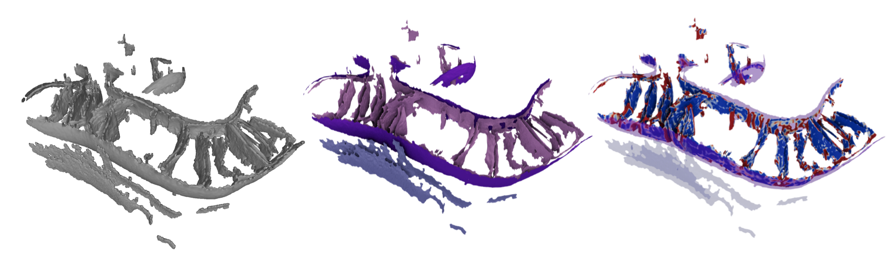
- Color by
curvedness_vvto see the curvature of the surface - Color by
OMM_dist(orIMM_dist) to see the distance from the IMM to the OMM or visa-versa
- Adjust color scales to see the features you are interested in. Add and edit the scalebar.
- Adjust the background, turn on ambient occlusion, and make the surfaces look nice for a screenshot.
- Take some nice pictures!
Generating some basic statistics and plots
python ../surface_morphometrics/single_file_histogram.py workdir/TE3_IMM.AVV_rh8.csv -n curvedness_vvwill generate an area-weighted histogram for a feature of interest in a single tomogram. I am using a variant of this script to respond to reviews asking for more per-tomogram visualizations!python ../surface_morphometrics/single_file_2d.py workdir/TE3_IMM.AVV_rh8.csv -n1 curvedness_vv -n2 OMM_distwill generate a 2D histogram for 2 features of interest for a single surface.
Running individual steps without pipelining
Individual steps are available as click commands in the terminal, and as functions
- Robust Mesh Generation
mrc2xyz.pyto prepare point clouds from voxel segmentationxyz2ply.pyto perform screened poisson reconstruction and mask the surfaceply2vtp.pyto convert ply files to vtp files ready for pycurv
- Surface Morphology Extraction
curvature.pyto run pycurv in an organized way on pregenerated surfacesintradistance_verticality.pyto generate distance metrics and verticality measurements within a surface.interdistance_orientation.pyto generate distance metrics and orientation measurements between surfaces.- Outputs: gt graphs for further analysis, vtp files for paraview visualization, and CSV files for pandas-based plotting and statistics
- Morphometric Quantification - there is no click function for this, as the questions answered depend on the biological system of interest!
morphometrics_stats.pyis a set of classes and functions to generate graphs and statistics with pandas.- Paraview for 3D surface mapping of quantifications.
Summary of File Types:
- Files with.xyz extension are point clouds converted, in nm or angstrom scale. This is a flat text file with
X Y Zcoordinates in each line. - Files with .ply extension are the surface meshes (in a binary format), which will be scaled in nm or angstrom scale, and work in many different softwares, including Meshlab.
- Files with surface.vtp extension are the same surface meshes in the VTK format. * The .surface.vtp files are a less cross-compatible format, so you can't use them with as many types of software, but they are able to store all the fun quantifications you'll do!. Paraview or pyvista can load this format. This is the format pycurv reads to build graphs.
- Files with .gt extension are triangle graph files using the
graph-toolpython toolkit. These graphs enable rapid neighbor-wise operations such as tensor voting, but are not especially useful for manual inspection. - Files with .csv extension are quantification outputs per-triangle. These are the files you'll use to generate statistics and plots.
- Files with .log extension are log files, mostly from the output of the pycurv run.
- Quantifications (plots and statistical tests) are output in csv, svg, and png formats.