Surface Morphometrics

Workflow Figure

Quantification of Membrane Surfaces Segmented from Cryo-ET or other volumetric imaging.

Surface morphometrics is a toolbox I developed during my postdoc to better understand how mitochondrial membranes remodel during stress. It turns out to be useful for a whole lot more than mitochondria! You can use it to assess aspects of membrane geometry in detail both locally and globally within cells, thanks to a robust meshing (modeling) algorithm and a set of simple tools for making measurements on the resulting surfaces.

Today we will scratch the surface with a single tomogram, but one of the most valuable aspects of building models and making quantifications is that it becomes possible to assess statistical significance by comparing quantifications across many tomograms in different cells and conditions. This is a powerful way to move from qualitative phenomenology about cellular remodeling to robust quantitative understanding of the underlying biology. With one tomogram, we're mostly still doing phenomenology.

New since 2024: one morphometrics command

The toolkit is now an installable package driven by a single morphometrics command with subcommands, instead of running python <script>.py directly. The old python script.py … calls still work for now via deprecation shims (they warn and forward), but please use the new commands. Two config keys were also renamed: data_dir → seg_dir and max_triangles → simplify_max_triangles. There are also two new capabilities since the workshop you may have seen before: optional mesh refinement (recentering vertices on the bilayer) and membrane thickness measurement.

Step 0: Set up the environment and the config file.

Activate the conda environment and check the install:

conda activate morphometrics                 # TODO: confirm env name
morphometrics --help                         # should list the pipeline subcommands

Move to the working folder for our project and generate a starter config:

cd /scratch/segmentation_dataset/morpho_run  # TODO: confirm path
morphometrics new_config                     # writes a fully-commented config.yml

Edit config.yml for our project's needs. I prefer Visual Studio Code for this! The key things to set:
- seg_dir: ./segmentations/ — folder containing your segmentation (label) MRC files.
- tomo_dir: ./tomograms/ — folder containing the raw tomogram MRC files (needed for thickness/refinement; each raw tomogram must share the basename of its segmentation).
- work_dir: ./morphometrics/ — folder for output files; exp_name is not currently used in this release.
- segmentation_values — the label-value → name mapping for your data. My mapping is as follows:
```
segmentation_values:
  IMM: 1     
  OMM: 2
  ER: 3
  PM: 4
  INM: 5
  ONM: 6
```
- cores — set to 24 to speed up computation today.
- Under surface_generation: leave isotropic_remesh: true and set target_area: 1.5. Generally, we recommend working with target_area around 1 nm² for good near-equilateral triangles (bigger = faster/coarser). Today, we're working a bit bigger to make sure the computation is fast, but finer meshes do better with thickness measurement and scanning.
- Under curvature_measurements: set radius_hit: 9 (the radius of the smallest feature of interest, in nm) and exclude_borders: 0.
- Under distance_and_orientation_measurements: list intra: [IMM, OMM, ER, PM, INM, ONM] and set inter: {OMM: [IMM, ER, PM, ONM], ER:[PM], ONM[INM]}. These are all the "interesting" interactions as far as I can tell.
- Under thickness_measurements: set average_radius: 20 (the radius for averaging the bilayer) and set it up for all your surfaces. Higher radius values will average over a larger area, which can be useful for smoothing out noise but may also obscure fine details.
- Under mesh_refinement: set iterations to 3, damping_factor: 0.95, xcorr_iterations: [1,2,3], and convergence_threshold to 0. This will use the faster xcorr mode, which locally sharpens membrane positions, for all of the iterations, rather than doing the much slower global positioning approach using a dual gaussian bilayer fit. For this curvature data, your global fits are probably very good, so this shouldn't be a big deal - but in the future, you may want to incorporate some dual gaussian steps at the end. I usually use 6 iterations, with the first 3 being xcorr and the rest being dual gaussian. This takes a long time, so I incorporate a convergence criteria (which we disable today) for when the meshes stop moving.

When you go back to your home institute, you can benchmark with example data before trying with yours

morphometrics fetch_example downloads a small cropped tomogram + segmentation from Zenodo into surface_morphometrics_example/ (with tomograms/, segmentations/, and a ready config.yml, IMM=1/OMM=2). Great for a dry run of the whole pipeline including thickness.

Step 1: Make Surface Meshes (Run time ~6 minutes on my machine)

Each step reads config.yml and writes into work_dir; every command prints a hint for the next one. Run them in order:

# 1. Segmentations -> surface meshes (screened Poisson + remeshing)
morphometrics make_meshes config.yml

This step will make meshes with mostly isotropic triangles of a target area of 1.5 nm². It outputs in two formats: a ply file that you can visualize and modify in meshlab, and a .surface.vtp file that is used for further processing and can be visualized in paraview. For now, lets take a look at your files in meshlab:

module load meshlab
meshlab morphometrics/*.ply

You can play around with the visualization here - try turning on the triangle edge display, or coloring by curvature. If we have time, I will walk through these, but if not we may move on quickly. Generally, you want to make sure you've had eyes on EVERY surface for at least a moment before proceeding through the rest of the pipeline - garbage in, garbage out, after all!

Step 2: Building a graph and measuring curvature robustly with `pycurv`. (Also ran in ~6 minutes on my machine)

In this step, we will use pycurv to build a graph and measure curvature using a vector voting algorithm. These graphs are what we use for all other operations going forward. Notably, the upstream pycurv software is great but quite slow; morphometrics uses a fork that has been extensively vectorized to deliver many-fold performance improvements.

morphometrics pycurv config.yml

The important output files from this step are the graph files (.AVV_rh9.gt) and the quantified surface files (.AVV_rh9.vtp). The graph can't be easily visualized, but the quantified surfaces can be loaded into paraview for analysis.

module load paraview
paraview morphometrics/YTC041_1_lam4_2_ts_002_labels_IMM.AVV_rh9.vtp

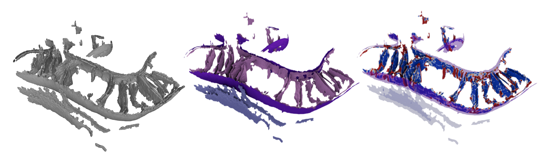
Try changing the visualization to "curvedness_VV" to see the curvature of the surface. Play around with color map settings and lighting. Ambient occlusion is a huge benefit for making nice figures, and changing the background to white is important for publication-quality images.

New since 2024. After pycurv and before distances/thickness, morphometrics refine_mesh config.yml recenters surface vertices onto the true bilayer center by sampling the raw tomogram density along surface normals. It improves every surface, but it is by far the slowest step (it re-runs pycurv internally each iteration), so be prepared for a longer than usual wait. We are doing a quicker version of it today that should be faster than normal.

export OMP_NUM_THREADS=1                             # This is a fix for a linux bug I ran into here at the workshop! 
morphometrics refine_mesh config.yml                 # writes *_refined_iter*.surface.vtp + convergence plots
morphometrics accept_refinement config.yml <step>    # promote the chosen iteration (use --dry-run to preview)

Try loading all of your refinement results into paraview to see the improvements. You can also look at the convergence plots to understand the refinement process. Usually you want to select the final step for moving forward, but you may not always want to! Make sure to check a surface in paraview before accepting it blindly! Focus in particular on ONM and INM - those should improve significantly.

Step 4: Distance and Thickness Measurement (Approximately 5 minutes for one tomogram)

The morphometrics distances_orientations config.yml command calculates the inter-membrane distance and orientation of the surfaces. This is one of the most useful steps for understanding membrane organization in situ, as membrane-membrane contact sites are a key regulatory feature across many biological processes.

morphometrics distances_orientations config.yml

Feel free to inspect your output files! Always be looking for interesting or unexpected patterns. Your eyes and brain make for fantastic neural nets!

Step 5: Thickness Measurement (Approximately 5 minutes for one tomogram)

Thickness measurement is done in two steps in morphometrics:

`morphometrics sample_density config.yml` # samples the raw tomogram density along surface normals.
`morphometrics measure_thickness config.yml` # calculates the thickness of the membrane.

This is another key metric for understanding membrane properties and can be used to analyze the impact of protein localization on membrane function - for instance, we have shown that prohibitin thins the membrane locally in mitochondrial inner membranes.

Thickness also automatically generates some summary statistics from the run - check out some of the generated png/svg files in the morphometrics output directory, as well as loading surfaces into paraview.

Step 6: Quick statistics and plots

One thing you may want to do with all your quantified surfaces is to generate histograms and 2D histograms to visualize the distribution of various morphological features. If you have lots of tomograms, you may also want to do some summary statistics - we aren't doing this today but we have the stats library for doing that! With that said, if you don't want to write python, just grab all our CSVs, load them into R studio or Excel or whatever your favorite tool for statistics is, and go to town!

morphometrics histogram YTC041_1_lam4_2_ts_002_labels_IMM.AVV_rh9.vtp -n curvedness_VV                  # area-weighted histogram
morphometrics hist2d  YTC041_1_lam4_2_ts_002_labels_IMM.AVV_rh9.vtp -n1 curvedness_VV -n2 OMM_dist     # area-weighted 2D histogram

Step 7 (Bonus round): Lets make some contextual structural biology figures!

Using morphometrics export_obj you can export the quantified surfaces as high-resolution OBJ files with color-coded features. These are compatible with lots of other softwares, including Blender, ChimeraX, and Surforama.

morphometrics export_obj config.yml YTC041_1_lam4_2_ts_002_labels_OMM.AVV_rh9.vtp --list-features      # see colorable arrays
morphometrics export_obj config.yml YTC041_1_lam4_2_ts_002_labels_OMM.AVV_rh9.vtp --feature IMM_dist --cmap magma

I have included instructions to make two great visualizations. Depending on time, we are going to do these both together:

Head to ChimeraX to make your own version of the cover figure from our JCB paper, but with more color
Head to Surforama to see how to use these OBJ files for locally visualizing membrane-associated proteins.

Not in this lesson:

morphometrics stats config.yml <name>   # assembles an Experiment pickle across all tomograms in the data folder

This is where multi-tomogram, multi-condition comparison happens — the heart of moving from phenomenology to statistics. With one tomogram there's not much to aggregate, so this mostly matters once you have a real dataset. Analysis from the pickle is done in pandas via the Experiment/Tomogram classes in surface_morphometrics.morphometrics_stats.

Under the hood / running individual modules

The pipeline steps wrap lower-level modules in the surface_morphometrics package, which you can also run directly with python -m surface_morphometrics.<module>:

Mesh generation (make_meshes): mrc2xyz (segmentation → point cloud) → xyz2ply (screened-Poisson reconstruction + masking) → ply2vtp (→ vtp for pycurv).
Morphology extraction: curvature (pycurv), refine_mesh/accept_refinement, intradistance_verticality + interdistance_orientation (wrapped by distances_orientations), sample_density + measure_thickness.

Summary of File Types

.xyz — point clouds (flat text X Y Z per line), nm or Å scale.
.ply — surface meshes (binary), nm or Å scale; open in Meshlab and many other tools.
.surface.vtp — the same meshes in VTK format; this is the input pycurv reads to build graphs. Open in Paraview / pyvista.
.AVV_rh*.vtp — pycurv outputs carrying the quantifications (the rh number is your radius_hit); richest for Paraview/pyvista visualization.
.gt — triangle graphs (graph-tool); fast neighbor operations, not for manual inspection.
.csv — per-triangle quantification tables; the files you use for statistics and plots.
.log — logs, mostly from pycurv.
Quantification outputs (plots/tests) are written as csv, svg, and png.

Parallelizing on a cluster

Most steps also accept a single input so you can run one tomogram/surface per job, e.g. morphometrics pycurv config.yml TE3_OMM.surface.vtp or morphometrics distances_orientations config.yml TE3.mrc. The pycurv and thickness steps are the slow ones; parallelizing them per tomogram is the way to scale to dozens of tomograms.