Surface Morphometrics in 2 Hours

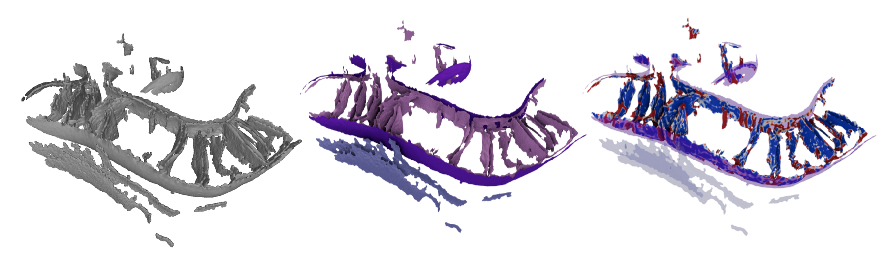
Quantifying membrane ultrastructure from a single cryo-ET tomogram — start to finish in one sitting.

Surface Morphometrics is a toolbox for building high-quality triangle-mesh models of membranes segmented from cryo-ET (or other volumetric imaging) and using them to measure membrane geometry — curvature, inter-membrane distance and orientation, and bilayer thickness — both locally and globally.

This is a condensed, single-page version of the full U Michigan tutorial. It is designed to run end-to-end in about two hours on a real tomogram. We work with one mitochondrial tomogram from EMPIAR-12534 and its pre-made segmentation, which contains just two membranes — the inner mitochondrial membrane (IMM) and outer mitochondrial membrane (OMM). Because there are only two surfaces and we keep the meshes a little coarse, every step finishes quickly.

What we skip to save time

The full workflow starts from a raw tomogram, segments membranes with MemBrain-seg, and cleans them up in Mosaic. Here we start from a pre-made IMM/OMM segmentation so we can spend all our time on the morphometrics itself. We also run a shortened mesh refinement (2 iterations instead of 6) and a coarser mesh than we would use for publication.

---

Installation

Install these before the session — the conda environment and the large downloads are the slow parts, and you don't want to spend your two hours on setup. Each tool lives in its own environment; that's normal for cryo-ET.

This workflow works on Mac and most Linux distributions. If you have a windows PC, either SSH into a workstation or set up Windows Subsystem for Linux. No GPU is required for any operations today.

Tool	Role today	How to install
Surface Morphometrics	Required — the whole pipeline	Conda (see below)
Paraview	Recommended — view quantified surfaces	Download
ChimeraX	Recommended — publication figures	Download
ArtiaX	Recommended — particles in tomogram context (ChimeraX plugin)	ChimeraX ▸ Tools ▸ More Tools… ▸ ArtiaX ▸ Install
Surforama	Recommended — pick membrane-associated proteins	pip install surforama in a fresh env
MorphometricsX	Optional — load quantified .vtp straight into ChimeraX	ChimeraX ▸ Tools ▸ More Tools… ▸ MorphometricsX ▸ Install

Surface Morphometrics (required)

git clone https://github.com/baradlab/surface_morphometrics.git
cd surface_morphometrics
conda env create -f environment.yml        # installs deps + the `morphometrics` command
conda activate morphometrics
morphometrics --help                        # should list the pipeline subcommands

On older Ubuntu (or if graph-tool fails to solve), use conda env create -f environment-ubuntu.yml instead. There is also a Docker image — see the repo README.

WSL users: fix git SSL first

On Windows Subsystem for Linux, git clone over HTTPS can fail with SSL certificate errors. Point git at the Windows certificate store once, before cloning:

git config --global http.sslbackend schannel

Surforama (recommended, for the last step)

Surforama is a napari plugin; install it into its own environment:

conda create -n surforama python=3.11
conda activate surforama
pip install surforama

ChimeraX add-ons (ArtiaX + optional MorphometricsX)

Install ChimeraX, then from inside ChimeraX open Tools ▸ More Tools… to reach the Toolshed and install ArtiaX (particles in context) and, optionally, MorphometricsX. Restart ChimeraX after installing. MorphometricsX opens the quantified .vtp surfaces directly and colors them by any stored field — a nice alternative to exporting OBJs, described in the ChimeraX bonus below. You can also install MorphometricsX from the command line: toolshed install ChimeraX-MorphometricsX.

---

Step 0: Download and organize the data

You need three files:

• Raw tomogram — EMPIAR file YTC041_1_lam4_2_ts_002.mrc_9.98Apx.mrc (~875 MB) from EMPIAR-12534. Needed for refinement and thickness. We save it locally as YTC041_1_lam4_2_ts_002.mrc (see the note below).
• Segmentation — YTC041_1_lam4_2_ts_002_labels.mrc (~437 MB), the matching IMM/OMM label map from the same EMPIAR entry.
• Ribosome picks — clean_ribosomes.star, a small STAR file used in the optional bonus at the end.

The pipeline expects the segmentation and tomogram in separate folders, with the tomogram sharing the segmentation's basename prefix. Grab the download_data.sh helper and run it:

# Download and lay everything out under ./morpho_run
curl -LO https://raw.githubusercontent.com/baradlab/morphometrics_2hr/main/download_data.sh
bash download_data.sh
cd morpho_run

Or do it by hand — the script simply runs these downloads into this layout:

mkdir -p morpho_run/tomograms morpho_run/segmentations morpho_run/star
cd morpho_run

EMPIAR=https://ftp.ebi.ac.uk/empiar/world_availability/12534/data/EMPIAR_upload

# Raw tomogram (~875 MB). Save WITHOUT the "_9.98Apx.mrc" double extension:
# the pipeline strips only the last extension to get a tomogram's basename, so
# "...ts_002.mrc_9.98Apx.mrc" would become "...ts_002.mrc_9.98Apx" and fail to
# match the "..._labels_<COMPONENT>" graph names during refinement/thickness.
curl -L -C - -o tomograms/YTC041_1_lam4_2_ts_002.mrc \
  "$EMPIAR/Reconstructed_tomograms/YTC041_1/YTC041_1_lam4_2_ts_002.mrc_9.98Apx.mrc"

# IMM/OMM segmentation (~437 MB)
curl -L -C - -o segmentations/YTC041_1_lam4_2_ts_002_labels.mrc \
  "$EMPIAR/Voxel_segmentations/YTC041_1/YTC041_1_lam4_2_ts_002_labels.mrc"

# Ribosome picks for the bonus step
curl -L -C - -o star/clean_ribosomes.star \
  https://baradlab.com/michigan_tutorial/latest/static/clean_ribosomes.star

The downloads are the slowest part of the day — kick them off first. When they finish you should have:

morpho_run/
├── tomograms/     YTC041_1_lam4_2_ts_002.mrc
├── segmentations/ YTC041_1_lam4_2_ts_002_labels.mrc
└── star/          clean_ribosomes.star

---

Step 1: Set up the environment and config

Activate the conda environment and confirm the CLI is available:

conda activate morphometrics          # use your morphometrics env name
morphometrics --help                  # should list the pipeline subcommands

Generate a starter config in the project folder and open it in your editor:

cd morpho_run
morphometrics new_config              # writes a fully-commented config.yml

Edit config.yml. For this two-membrane, two-hour run the important keys are below — everything else can stay at its default:

seg_dir: "./segmentations/"     # folder with the label MRC
tomo_dir: "./tomograms/"        # folder with the raw tomogram (for refinement + thickness)
work_dir: "./morphometrics/"    # all outputs land here

segmentation_values:            # this segmentation only has two membranes
  IMM: 1
  OMM: 2

cores: 8                        # bump this up if you have more cores

surface_generation:
  isotropic_remesh: true
  target_area: 1.5              # nm^2 per triangle; coarse-ish so meshing is fast today
                                # (use ~1.0 for publication-quality meshes)

curvature_measurements:
  radius_hit: 9                 # radius (nm) of the smallest feature of interest
  exclude_borders: 0

distance_and_orientation_measurements:
  intra: [IMM, OMM]
  inter:
    OMM: [IMM]                  # OMM<->IMM is the only inter-membrane pair here

thickness_measurements:
  average_radius: 12            # small radius keeps real thickness signal
  components: [IMM, OMM]

mesh_refinement:                # SHORTENED for today: 2 iterations total
  iterations: 2
  xcorr_iterations: [1]         # iter 1 = fast cross-correlation, iter 2 = dual-Gaussian fit
  convergence_threshold: 0      # 0 = never stop early, so both iterations run

If your computer has fewer than 8 cores, reduce accordingly.

Confirm your base settings are finding everything properly by running:

morphometrics validate config.yml

Why these refinement settings

The full pipeline usually runs 6 iterations (the first few cross-correlation, the rest dual-Gaussian). Refinement is by far the slowest step because it re-runs pycurv internally each iteration. Setting iterations: 2 with xcorr_iterations: [1] gives you exactly one cross-correlation pass (fast, locally sharpens the bilayer) followed by one dual-Gaussian pass (precise global centering) — enough to see the method work without the long wait. convergence_threshold: 0 forces both iterations to run even if the mesh barely moves.

---

Step 2: Make surface meshes (~8 minutes)

morphometrics make_meshes config.yml

This converts each labeled membrane into a surface mesh (screened-Poisson reconstruction + isotropic remeshing). It writes two formats per surface: a .ply for viewing in mesh editors and a .surface.vtp used by the rest of the pipeline. You get one of each for IMM and OMM.

Take a quick look before going further — garbage in, garbage out. Open the .surface.vtp meshes in Paraview (the same tool you'll use for the quantified surfaces later):

paraview morphometrics/YTC041_1_lam4_2_ts_002_labels_OMM.surface.vtp

Make sure both membranes look like clean, continuous surfaces. Set the representation to Surface With Edges to see the individual triangles, and load the IMM .surface.vtp alongside the OMM to inspect them together.

---

Step 3: Measure curvature with pycurv (~15 minutes)

morphometrics pycurv config.yml

pycurv builds a triangle graph and measures curvature robustly with a vector-voting algorithm (morphometrics uses a heavily vectorized fork for speed). The key outputs per surface are the graph (.AVV_rh9.gt), the quantified surface (.AVV_rh9.vtp), and a per-triangle table (.AVV_rh9.csv).

Load a quantified surface in Paraview and color by curvedness_VV:

paraview morphometrics/YTC041_1_lam4_2_ts_002_labels_IMM.AVV_rh9.vtp

The IMM should show its characteristic high-curvature cristae; the OMM should be much smoother.

---

Step 4: Refine the meshes (~20 minutes today)

Refinement recenters surface vertices onto the true bilayer center by sampling the raw tomogram density along each surface normal. It runs after pycurv and before distances/thickness. We shortened it to two iterations (one cross-correlation, one dual-Gaussian):

export OMP_NUM_THREADS=1                            # avoids a threading bug on some Linux setups
morphometrics refine_mesh config.yml                # writes *_refined_iter1/2 + convergence plots

No graph files found matching ... ?

If refinement (or thickness) prints something like No graph files found matching: ./morphometrics/YTC041_1_lam4_2_ts_002.mrc_9.98Apx*OMM.AVV_rh9.gt, your tomogram still has the EMPIAR double extension. The pipeline strips only the last .mrc, leaving ...ts_002.mrc_9.98Apx, which doesn't match the ..._labels_<COMPONENT> graph names. Rename it to a clean single extension and re-run:

mv tomograms/YTC041_1_lam4_2_ts_002.mrc_9.98Apx.mrc tomograms/YTC041_1_lam4_2_ts_002.mrc
morphometrics refine_mesh config.yml

The updated download_data.sh already saves it as YTC041_1_lam4_2_ts_002.mrc, so fresh downloads won't hit this.

Inspect the convergence plots and the per-iteration surfaces in Paraview, then promote the iteration you like (usually the last one):

morphometrics accept_refinement config.yml 2 --dry-run   # preview what would be promoted
morphometrics accept_refinement config.yml 2             # commit iteration 2

accept_refinement re-points the working files at the chosen iteration. Because we accepted a fully-refined iteration, you're ready to continue directly to distances.

---

Step 5: Distances and orientations (~4 minutes)

morphometrics distances_orientations config.yml

This measures inter-membrane distance and relative orientation between OMM and IMM, plus intra-surface verticality for each. Membrane–membrane spacing is one of the most biologically informative metrics you can pull from a tomogram — here it captures how tightly the IMM tracks the OMM. Outputs are added as new columns in the per-surface CSVs and as arrays on the VTP surfaces.

---

Step 6: Membrane thickness (~4 minutes)

Thickness is a two-command step: sample the density along normals, then fit the bilayer profile.

morphometrics sample_density config.yml       # samples raw tomogram density along normals
morphometrics measure_thickness config.yml    # fits the bilayer to estimate thickness

measure_thickness also writes summary PNG/SVG plots into the output folder — open a couple of them, and load a surface in Paraview colored by thickness to see the local variation across the IMM and OMM.

---

Step 7: Quick plots

Every quantified surface has a .csv you can histogram directly. A couple of examples:

# Area-weighted 1D histogram of IMM curvedness
morphometrics histogram morphometrics/YTC041_1_lam4_2_ts_002_labels_IMM.AVV_rh9.csv -n curvedness_VV

# Area-weighted 2D histogram: IMM curvedness vs. distance to the OMM
morphometrics hist2d morphometrics/YTC041_1_lam4_2_ts_002_labels_IMM.AVV_rh9.csv \
  -n1 curvedness_VV -n2 OMM_dist

The CSVs are plain per-triangle tables — if you'd rather not write Python, load them into R, Excel, or your favorite stats tool and go from there. With one tomogram this is mostly phenomenology; the real power of the method comes from aggregating these quantifications across many tomograms and conditions (morphometrics stats), which we don't cover today.

---

Step 8: Measure distances from particles to the membrane

The quantified surfaces are also a ruler for particles. Given a STAR file of coordinates, morphometrics generate_patches finds the nearest membrane triangle to each particle and annotates the STAR with a per-particle mesh_distance (in nm). This is exactly how you separate, say, membrane-associated (co-translating) ribosomes from free cytoplasmic ones. We'll use the clean_ribosomes.star file you downloaded and measure each ribosome's distance to the OMM.

Command name

The tool is generate_patches — it can also carve out membrane patches around each particle and matched random controls, but today we only want the distance annotation, so we turn the patch/control machinery off.

Time to edit the patch_analysis block to your config.yml. The particle coordinate settings already match this STAR (rlnCoordinateX/Y/Z in pixels, rlnPixelSize = 3.33 Å/px), so the two keys that matter today are annotate_star: true and generate_random: false:

patch_analysis:
  membrane_label: OMM                    # measure ribosome distance to the outer membrane
  annotate_star: true                    # write mesh_distance back into the STAR
  generate_random: true                  # no random control patches today
  particle_max_distance: null            # keep every particle; we just want distances
  star_dir: "./star/"                    # where the STAR lives
  star_pattern: "clean_ribosomes.star"   # our file isn't named <tomogram>.star, so give it literally
  # coordinate columns / pixel size use the defaults, which fit this STAR:
  # star_coord_columns: [rlnCoordinateX, rlnCoordinateY, rlnCoordinateZ]
  # star_pixelsize_column: rlnPixelSize
  # star_coords_in_pixels: true

Then run:

morphometrics generate_patches config.yml
morphometrics patch_statistics config.yml

It picks up the OMM graph from Step 3/4 and writes an annotated STAR to the output folder:

morphometrics/clean_ribosomes_OMM_meshannotated.star

Each row keeps its original particle data plus three new columns: mesh_distance (nm to the nearest OMM triangle), patch_id (the 1-based row number, so it maps straight back to the original STAR), and mesh_neighbor_id (the index of that nearest triangle). Sort or filter on mesh_distance to pull out the membrane-proximal ribosomes — e.g. everything within ~15 nm of the OMM — and carry that filtered STAR into the visualization steps below.

---

Bonus: contextual figures in ChimeraX

If you finish early, the quantified surfaces make great figure material. In ChimeraX, with the ArtiaX plugin, you can render a colored membrane surface with the ribosomes sitting in their real positions.

Get a colored surface into ChimeraX. You have two options:

Option A — export a colored OBJ. Bake a feature into a colored high-resolution OBJ. ArtiaX and ChimeraX work in Ångström, which is export_obj's default (--scale_to_angstroms true), so no scale flag is needed here:

# see the colorable arrays
morphometrics export_obj config.yml \
  morphometrics/YTC041_1_lam4_2_ts_002_labels_OMM.AVV_rh9.vtp --list-features

# Ångström-scaled OBJ for ChimeraX/ArtiaX, written to obj_angstrom/
morphometrics export_obj config.yml \
  morphometrics/YTC041_1_lam4_2_ts_002_labels_OMM.AVV_rh9.vtp \
  --feature IMM_dist --cmap magma \
  --scale_to_angstroms true --output-dir obj_angstrom/

Each run writes <base>_<feature>.obj (plus its .mtl and .png), so this produces obj_angstrom/YTC041_1_lam4_2_ts_002_labels_OMM.AVV_rh9_IMM_dist.obj. open that .obj in ChimeraX. (The scale is baked into the file's coordinates — that's why we make a separate nm-scaled OBJ for Surforama below.)

Option B — MorphometricsX (no export needed). If you installed the optional MorphometricsX bundle, skip export_obj entirely: open morphometrics/YTC041_1_lam4_2_ts_002_labels_OMM.AVV_rh9.vtp directly and use the MorphometricsX panel to color by any stored field (curvedness, thickness, IMM_dist, …), adjust the colormap/range, and add a color key — all interactively. This is usually the faster and more flexible route for ChimeraX figures, since you can flip between quantifications without re-exporting. Note the mesh is stored in nm, so set the panel's Scale to 10 to line it up with an Ångström-scale tomogram and particle list.

Add the ribosomes. The clean_ribosomes.star file you downloaded holds oriented ribosome picks for this tomogram:

1. Load the OBJ (Option A) or the .vtp (Option B) as your surface.
2. Launch ArtiaX and add star/clean_ribosomes.star to the particle lists.
3. Under Select/Manipulate, set the Pixel Size factors to 3.3, 1.
4. Add the raw tomogram to the ArtiaX tomogram list and average ~5 slabs for a clean orthoslice (or hide it).
5. Fetch a ribosome map (e.g. open 48752 from emdb), add it as a new surface for the particle list, enable soft lighting, and make your figure.

---

Bonus: exploring proteins on the surface with Surforama

Surforama is a napari plugin that projects the local tomogram density onto a membrane mesh, so you can see what sits on the membrane, pick particles directly on the surface (oriented along the surface normal), and export them as RELION STAR files for subtomogram averaging. It pairs naturally with the surfaces you just built.

Make an nm-scaled surface for Surforama. Surforama matches the mesh to the tomogram in nanometers, so export with --scale_to_angstroms false (the opposite of the Ångström OBJ we made for ChimeraX). Write it to its own folder so the two OBJs don't overwrite each other — the filenames don't encode the scale:

morphometrics export_obj config.yml \
  morphometrics/YTC041_1_lam4_2_ts_002_labels_OMM.AVV_rh9.vtp \
  --feature curvedness_VV \
  --scale_to_angstroms false --output-dir obj_nm/

This writes obj_nm/YTC041_1_lam4_2_ts_002_labels_OMM.AVV_rh9_curvedness_VV.obj.

Optional but helpful — deconvolve the tomogram so densities read more clearly (needs IMOD's mtffilter):

# write it to the project root, NOT tomograms/, so the pipeline's *.mrc glob won't pick it up
mtffilter tomograms/YTC041_1_lam4_2_ts_002.mrc -dec 0.5 -def 5 YTC041_1_lam4_2_ts_002_dec.mrc

Launch Surforama with the tomogram and the mesh:

conda activate surforama
surforama \
  --image-path YTC041_1_lam4_2_ts_002_dec.mrc \
  --mesh-path obj_nm/YTC041_1_lam4_2_ts_002_labels_OMM.AVV_rh9_curvedness_VV.obj

Adjust the projection offset and thickness — around an offset of 5–8 you should find dark spots on the outer membrane that correspond to membrane-associated ribosomes. To pick them:

1. Click Enable under "pick on surface".
2. Click points on the surface where you see ribosomes.
3. Click Select File next to the file path and choose a STAR filename.
4. Click Save.
5. Inspect the picks — they get initial orientations from the surface normals, so you get phi/psi for free (with rot at ±180). That geometric head start is exactly what makes membrane-anchored particles nice to average.

---

File types you'll see

Extension	What it is
.mrc	tomogram / segmentation volumes
.ply	surface mesh for viewing/editing (Meshlab)
.surface.vtp	surface mesh in VTK format; input to pycurv
.AVV_rh9.vtp	pycurv output carrying the quantifications (rh = radius_hit); best for Paraview
.AVV_rh9.gt	triangle graph (graph-tool); fast, not for manual inspection
.AVV_rh9.csv	per-triangle quantification table; use for stats and plots
.png / .svg	summary plots generated by the pipeline

---

Condensed from the U Michigan CryoET Segmentation & Modeling Tutorial. Surface Morphometrics was developed by Ben Barad in Danielle Grotjahn's lab and is maintained by the Barad lab.